What Limits AI Training Compute, and How Does It Scale?

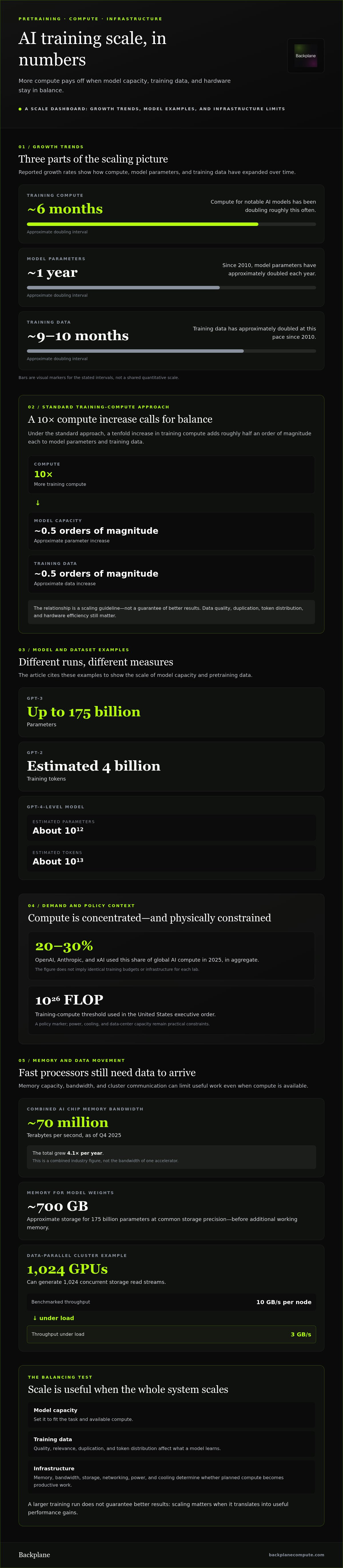
More compute only pays off when the model, data, and hardware scale together. Training compute for notable AI models has been doubling roughly every six months, but scaling AI training compute does not guarantee better results. Gains depend on how efficiently a system uses its data and hardware, and whether continued training improves performance.

It’s easy to focus on model size or GPU count. The harder question is whether additional compute is matched by enough high-quality pretraining data, sufficient memory and bandwidth, and infrastructure that keeps large clusters working efficiently. If these elements fall out of balance, extra resources can increase costs without delivering proportionate progress.

This article explains how pretraining connects model size, data, and compute, then explores the physical and economic limits that shape scale. You’ll see why efficiency and convergence matter, how training differs from deployment, and which infrastructure constraints determine whether a larger training run delivers meaningful gains.

Pretraining scaling and the relationship between data, model size, and compute

Pretraining scaling means increasing the compute used to expose a model to data and adjust its parameters. Scaling AI training compute works best when model capacity, dataset size, and hardware stay in balance.

Scaling laws describe how performance changes as training compute, model size, and data increase together. Under the standard training-compute approach, a tenfold compute increase adds roughly 0.5 orders of magnitude each to model parameters and training data. Training compute for notable AI models has doubled roughly every six months. Since 2010, model parameters have approximately doubled every year, while training data has doubled every nine to ten months.

These trends have produced models with billions or trillions of parameters and pretraining datasets containing trillions of tokens. GPT-3 had up to 175 billion parameters. GPT-2 was estimated to use 4 billion training tokens, while a GPT-4-level model is estimated at about 10¹² parameters and 10¹³ tokens. More data alone is not enough: duplication, quality, and token distribution influence what the model learns.

Mixture-of-Experts (MoE) models manage capacity differently. Mixture-of-Experts models can route each token through only some of their experts, rather than activating the entire model. In healthcare, reasoning models can support analysis of clinical information; in retail, they can interpret product and customer data; in logistics, they can compare routes and constraints. Each application depends on relevant training data and reliable evaluation, not parameter count alone.

Steps in Scaling a Training Run

Scaling a training run means expanding the model, dataset, and compute while coordinating each stage. Define the task and prepare representative data first. Then set model capacity and compute, distribute training across GPUs, and evaluate progress. This sequence matters because a larger run can amplify data weaknesses or infrastructure bottlenecks instead of improving useful capabilities.

Training Infrastructure and Resource Requirements

Large-scale training infrastructure combines GPUs, fast data movement, power, cooling, and data-center capacity. The required GPU count depends on model size, sequence length, training duration, and each accelerator’s effective utilization. Energy and cooling must support sustained operation, while storage and networking need to deliver data without leaving processors idle. These constraints determine whether a planned compute budget translates into productive training.

GPU prices and training costs vary with hardware choice, capacity, utilization, power, and operating arrangements. A project’s price depends on its specific requirements and is provided after a quote request. There is no single GPU count or compute total that applies to every frontier model; architecture, data volume, and training objectives determine the requirement.

Comparing AI Labs’ Training Compute

Public comparisons are clearest at the aggregate level: OpenAI, Anthropic, and xAI used 20-30% of global AI compute in 2025. That figure indicates concentrated demand, but it does not establish an identical training budget or infrastructure design for each lab. Compare runs by compute, model architecture, data, and evaluation results, rather than parameter totals alone.

In the United States, the executive order uses a training-compute threshold of 10²⁶ FLOP. That threshold is one policy marker for large-scale training; compute planning also has to account for the physical limits of power, cooling, and data-center infrastructure.

Chip, memory, and packaging constraints

Accelerator performance depends on more than processing speed. Memory capacity and bandwidth, chip packaging, and communication between GPUs determine how much useful work a training or inference system can sustain. A chip may offer substantial compute capability yet spend valuable cycles waiting for data.

Memory bandwidth sets the rate at which processors can access model weights and intermediate values. Total AI chip memory bandwidth grew 4.1x per year and reached roughly 70 million terabytes per second as of Q4 2025. That global figure reflects the combined industry, not the bandwidth of one accelerator. For individual systems, the balance between compute and local memory bandwidth affects throughput.

Model weights also create a direct memory requirement. At common storage precision, 175 billion parameters occupy roughly 700 GB before accounting for additional working memory. During inference, the KV cache stores attention keys and values from earlier tokens so the model can reuse context. Longer inputs and larger batches increase cache demand, potentially crowding out other data. Cache allocation, batching, and lower-precision representations are techniques that help optimize memory use, though each involves system and quality trade-offs.

Packaging connects compute dies with high-bandwidth memory and affects how efficiently data moves within an accelerator. Advanced packaging can place components closer together, but physical design, heat removal, and manufacturing capacity constrain the configurations available. At rack scale, GPU clusters also rely on network links to synchronize distributed work and storage systems to feed training data.

Clusters, networking, and storage affect scale by determining whether GPUs receive data and exchange results without costly stalls. For example, a 1,024-GPU data-parallel cluster can generate 1,024 concurrent storage read streams; throughput that benchmarks at 10 GB/s per node may fall to 3 GB/s under load.

Inference hardware faces related but distinct pressures. It must repeatedly move model weights and KV-cache data while serving requests, so memory bandwidth and capacity can limit token generation even when processors have unused compute. Batching can improve utilization, but larger batches also increase memory demand and may affect response times.

These constraints make infrastructure design a systems decision, not a chip-count exercise. Teams assessing compute sites can weigh power, cooling, networking, and storage alongside accelerator capacity; compute infrastructure planning connects those requirements to viable facilities.

Deployment versus pre-training compute costs

Pre-training concentrates compute into a defined run; deployment spreads it across every user request. As models enter production, inference is estimated to consume 80-90% of lifecycle resources. Stanford AI Index 2025 notes that inference costs now dominate training costs for most enterprises. The operational question shifts from how much compute built the model to how often it runs, how long prompts are, and how much reasoning each task requires.

Inference has two distinct stages. During prefill, the model processes the prompt, and attention has a quadratic cost relative to input length. During decode, the model generates output one token at a time. Longer conversations require more processing and memory for accumulated context. Runtime efficiency therefore depends on request length, batch size, hardware utilization, and the model’s output patterns. Optimizing one factor can shift pressure to another, such as memory use or response time.

Reasoning adds another variable. For challenging queries, inference can require over 100 times the compute of a single traditional LLM pass. A system might allocate 1,000 times normal inference compute to a difficult mathematics problem, while using the usual amount for intuitive questions. This selective allocation can improve performance without applying the larger compute budget to every request. At scale, however, even a twofold increase in compute for every question changes the total operating workload.

A practical comparison weighs total deployment compute against the pre-training run. Under rough GPT-4-level arithmetic, deployment compute overtakes pre-training once total generated deployment tokens exceed total training tokens. The same estimate places the crossover beyond 10¹⁰ deployments at 10³ inference steps per deployment. These are model-specific estimates, not universal thresholds: usage volume and reasoning intensity determine how quickly cumulative inference catches up.

To compare workloads across a portfolio, the article’s rough effective-compute measure adds pre-training orders of magnitude to 0.7 times inference orders of magnitude. One order of magnitude more inference compute on a task can improve performance about as much as 0.5 to 1 orders of magnitude more pre-training compute. That makes inference a potential source of capability, not merely a serving expense. Scaling AI training compute should therefore be evaluated alongside expected runtime demand.

For planning, separate workloads by task difficulty, prompt length, and expected output. Estimate how often each workload runs and whether it needs ordinary inference or extended reasoning. This helps identify where batching, model choice, or selective compute allocation can improve efficiency. The key distinction: pretraining creates learned capacity, while production usage determines how much compute the resulting model consumes over time.

AI compute scaling versus efficiency

More compute expands what a system can learn, but efficiency determines how much progress each unit delivers. A larger language model may produce stronger results, while a more efficient training or inference strategy may achieve similar capabilities with fewer resources. Compare both dimensions before treating infrastructure growth as the only way forward.

Hardware efficiency improves over time, but not at the pace of demand. GPU computing speed has doubled roughly every 2.5 years per dollar spent. Meanwhile, since Colossus 1 launched in August 2024, the record for the largest AI data center has doubled every seven months. That contrast shows why operators cannot rely on chip advances alone. Site capacity, power delivery, and system utilization all influence the compute available for learning.

Efficiency also means reusing a foundation model effectively. Developing derivative models for different use cases could require around 30 times more compute than pretraining the original foundation model. That workload can include adaptation, evaluation, and maintaining specialized versions. The trade-off is operational: a portfolio of narrower models can better serve specific tasks, but each model adds compute needs. Teams should compare the cost of that model ecosystem with the value of its capabilities.

Inference provides another path to performance. In one example, a model trained with 10²⁴ FLOP could be scaled by 4 orders of magnitude at inference to perform at the level of a model trained with 10²⁷ FLOP. This illustrates how targeted test-time compute can sometimes substitute for a larger pretraining run. The method suits tasks where extra reasoning improves the answer, not every routine request.

Efficiency gains also depend on the workload. A reasoning model may use additional compute to explore alternatives before answering, while a simpler request may need only a direct response. Allocating resources by task can make better use of available hardware than applying the same compute budget uniformly. Measure results against the task’s quality requirements, response needs, and total workload.

Physical expansion remains a constraint. Bain & Company estimates U.S. data centers could need 100 gigawatts of additional power by 2030, and projects half a trillion dollars a year in investment to meet data-center demand. These figures frame the infrastructure challenge: scaling requires viable power and facilities, while efficiency reduces wasted capacity. The strongest strategy combines both, matching new compute supply to workloads where additional resources create measurable progress.

Training compute and convergence

Convergence is the point where additional training produces progressively smaller gains on a chosen measure. It changes the central question from “How much compute can this run use?” to “What new capability does the next increment deliver?” A figure cited for AI training illustrates compute scaling by a factor of 10,000 without reaching a plateau. That does not mean every added operation creates equal progress. Operators must track useful outcomes, not compute volume alone.

Training compute doubled roughly every two years from 1950 to 2010. That long-run pattern shows how rapidly the available ceiling can move, but it cannot predict whether a particular run will converge efficiently. Loss curves can show whether a model is still learning patterns from its training data. Evaluation results reveal whether that learning transfers to real tasks, including reasoning or production workloads. If training loss improves while task performance stalls, more compute may not solve the actual problem.

Cluster behavior can obscure this distinction. A 32-node AI cluster may run cleanly, then stall when expanded to 256 nodes. At that scale, communication, synchronization, and workload balance can consume the gains expected from additional hardware. Engineers should compare throughput and training progress as nodes are added, then locate where communication or coordination becomes the limiting factor. A larger cluster is useful only if it advances training at a corresponding pace.

Topology choices also change with scale. A 64-node cluster can tolerate network arrangements that a 1,024-node cluster cannot. As ai systems expand, small communication delays can affect more devices and hold up collective operations. This creates a practical convergence issue: if each training step takes longer because the cluster is poorly matched, the model may use more elapsed time without learning proportionately more. Cluster performance belongs in the same review as model metrics.

To assess convergence, connect three signals: training progress, evaluation performance, and cluster throughput. For example, if a reasoning benchmark stops improving while each training step slows after a scale-up, adding nodes alone will solve neither problem. The team needs to find out whether the bottleneck comes from data quality, model behavior, or infrastructure operations. Each cause requires a different response, so a single compute total cannot predict the result.

Treat compute as an input, not an outcome. Before expanding a run, define which capability should improve, select evaluations that measure it, and establish how infrastructure throughput will be monitored. Then compare added compute with measured gains. This makes scaling decisions evidence-based: continue while learning remains productive, and redirect resources when model progress or cluster operations plateau.

Backplane: GPUs-as-a-Service

Backplane connects AI compute demand with infrastructure suited to training and deployment workloads. Teams that need GPU capacity without developing a dedicated site can use GPUs-as-a-Service. For sustained or larger requirements, Dedicated Financed Sites provide a route to dedicated infrastructure, while Property Viability Assessment and Infrastructure Financing Structuring address site potential and project financing.

The right path depends on workload scale, power needs, facility readiness, and the level of control the operation requires. If access to compute or suitable infrastructure constrains your training plans, assess these requirements before committing to a deployment model.

Contact Backplane to discuss your compute infrastructure requirements.

Turn Compute Plans Into an Infrastructure Decision

Turn your training roadmap into an infrastructure decision. Define the workload to support, the capacity it requires, and the operating model that fits your project. This gives you a practical basis for scaling AI training compute without treating growth as an end in itself.

Backplane offers GPUs-as-a-Service for GPU capacity, Dedicated Financed Sites for dedicated infrastructure, and Property Viability Assessment to evaluate site potential. These options connect compute requirements with the infrastructure path suited to the project.

Bring your requirements into focus and determine a clear direction for your next phase. Contact Backplane to discuss your compute needs. Your next infrastructure decision can start with a defined workload and a plan built around it.

Frequently Asked Questions

What Is Pretraining Scaling?

Pretraining scaling means expanding the resources used to teach a model general-purpose patterns before adapting it to a specific task. A language model, for example, can learn by predicting the next token across a broad text corpus. Teams can increase dataset coverage, model capacity, or training compute, then test whether the model transfers to tasks it was not specifically trained to perform. This stage builds the foundation for later adaptation.

What is AI compute scaling?

AI compute scaling means expanding computing resources to support more demanding AI workloads. This can involve adding accelerators to training, distributing work across more machines, or assigning more compute to inference. For example, a company serving document analysis may need to scale inference as request volume grows, even after the model’s training run is complete. The relevant measure is useful workload capacity, not hardware count alone.

What is scaling in AI models?

Scaling an AI model means changing its size, training exposure, or operating resources to increase its capabilities. A team might widen a model, train it on a broader dataset, or adapt a foundation model for legal document review. These choices affect different outcomes: architecture changes capacity, data changes the examples available for learning, and adaptation targets a specific use. Evaluation on the intended task helps show which change matters.

What does scaling AI training compute mean?

Scaling AI training compute means allocating more processing to a training run, often by changing accelerator capacity, training duration, or distributed execution. The goal is to improve a defined capability, not simply maximize operations. For example, a team training a code model could test whether added compute improves performance on held-out programming tasks. Evaluation helps distinguish useful progress from a larger run that increases infrastructure demand without solving the target problem.

How does model performance change as training compute increases?

Model performance often improves as training compute rises, but gains can diminish and vary by task. A model may become more accurate on broad language tests yet still make errors in a specialized workflow. Track separate measures, such as answer accuracy, reliability, and task completion, using examples kept outside the training data. If these measures stop improving, the next investment may be better data, a revised objective, or targeted adaptation rather than more compute.

What are the compute and data scaling laws for AI training?

Compute and data scaling laws are empirical relationships describing how model performance changes with training compute, dataset size, and model size. They help teams estimate promising allocations, but they are guides, not guarantees for every architecture or dataset. A run trained on repeated or poorly matched examples, for instance, may yield less value than one using relevant, varied material. Validation data tests whether a projected relationship holds for the task.

How should compute, training data, and model size be balanced?

Balance these resources against the task and the quality of available data. Start with the capability the model must deliver, then assess whether the dataset contains relevant, diverse examples and whether the model can learn from them. A specialized support model may benefit more from carefully curated product documentation than from a much larger general corpus. Use validation results to determine whether errors stem from insufficient examples, model capacity, or training execution before expanding any one resource.

What are the main risks and bottlenecks when scaling AI training compute?

Key risks include weak or duplicated training data, unstable optimization, equipment failures, and inadequate recovery planning. A long run can lose progress if checkpoints are infrequent or stored where failures could affect them. Evaluation can also mislead when test examples overlap with training material. Before scaling up, assess data integrity, monitor training stability, test checkpoint restoration, and track whether evaluation results reflect the intended real-world task.